Coarse-to-Fine

Formal definition

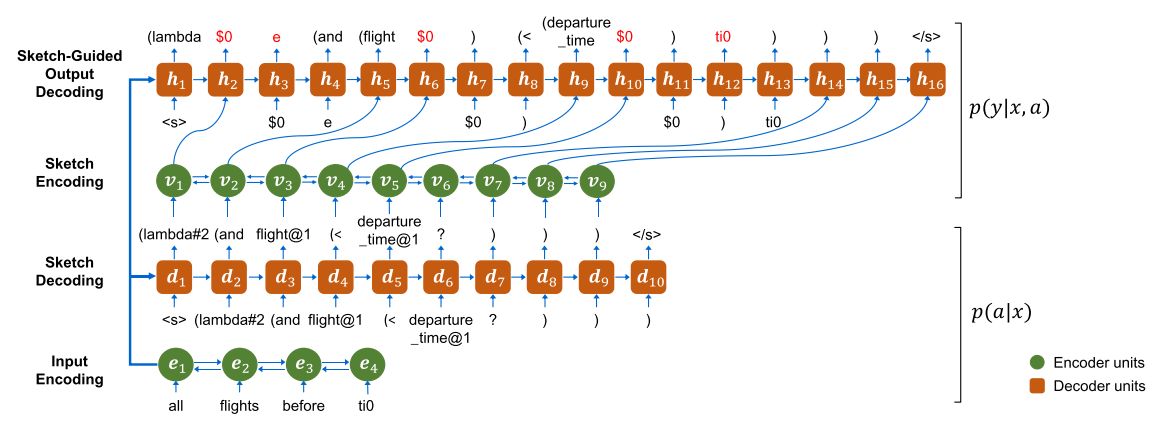
The input of the model consists of a sequence $\mathbf{x} = x_1, x_2, \dots, x_N$ where each $x_i$ is natural language utterance, such as $\mathbf{x} = \{ \texttt{call, the, function, func} \}$ . The final output (i.e. code tokens) is represented as a sequence $\mathbf{y} = y_1, y_2, \dots, y_M$ . The goal is to estimate the probability of generating the sequence $\mathbf{y}$ , given the input $\mathbf{x}$ , i.e. $p(\mathbf{y} \vert \mathbf{x})$ , while considering the sketch $\mathbf{a} = a_1, a_2, \dots, a_S$ . Therefore, the probability is factorized as

$p(\mathbf{y} \vert \mathbf{x}) = p(\mathbf{y} \vert \textbf{x}, \textbf{a}) \cdot p(\mathbf{a} \vert \textbf{x})$

where

$\begin{align*} p(\mathbf{a} \vert \textbf{x}) = \prod_{t=1}^{\vert\mathbf{a}\vert} p(a_t \vert a_{<t}, \mathbf{x})\\ p(\mathbf{y} \vert \textbf{x}, \textbf{a}) = \prod_{t=1}^{\vert\mathbf{y}\vert} p(y_t \vert y_{<t}, \mathbf{x}, \mathbf{a}) \end{align*}$

We see that the generation of the next token fully depends on the previously generated tokens of the same kind. For the final output, the entire sketch is also considered. This factorization clearly emphasizes the two-step process.

The $\textbf{input encoder}$ , modeled as a bi-directional recurrent neural network with LSTM units, produces vector representations of the natural language input $\mathbf{x}$ , by applying a linear transformation corresponding to an embedding matrix $\mathbf{E}$ over the one-hot representation of the token: $\mathbf{x_t} = \mathbf{E} \cdot \mathbf{o}(x_t)$ Specifically, each word is mapped to its corresponding embedding (e.g. GloVe word embeddings). The output of the encoder is $\mathbf{e}_t = \left[ \overrightarrow{\mathbf{e}_t}, \overleftarrow{\mathbf{e}_t} \right]$ , which denotes the concatenation of the forward and backward passes in the LSTM function. The motivation behind a bi-directional RNN is to be able to construct a richer hidden representation of a word vector, making use of both the forward and backward contexts.

The $\textbf{sketch decoder}$ is also a RNN with LSTM cells. Furthermore, an attention mechanism for learning soft alignments is used. An attention score $s_{tk}$ , which $\textit{measures}$ the contribution of each hidden state, is computed, corresponding to the $t$ -th timestep, on the $k$ -th encoder hidden state, where $\textbf{d}_t$ is the hidden state of the decoder. Thus, at each timestep $t$ we get a probability distribution over the hidden states of the encoder:

$s_{tk} = \frac{\exp(\mathbf{d}_t \cdot \mathbf{e}_k)}{\sum_{k=1}^{\vert\mathbf{x}\vert} \exp(\mathbf{d}_t \cdot \mathbf{e}_j)}$

with

$\sum_k s_{tk} = 1$

Now we can compute the probability of generating a sketch token $a_t$ for the current timestep:

$p(a_t \vert a_{<t}, \mathbf{x}) = \text{softmax}_{a_t} \left( \mathbf{W_o} \mathbf{d}_t^{\textit{att}} + \mathbf{b_o}\right)$

where

$\mathbf{e}_t^d = \mathbb{E}_k\left[ \mathbf{e}_k \right] = \sum_{k=1}^{\vert\mathbf{x}\vert} s_{tk} \cdot \mathbf{e}_k$

is the expected value of the hidden state vector for timestep $t$ , and

$\textbf{d}_t^{\textit{att}} = \tanh \left( \textbf{W}_1 \cdot \textbf{d}_t + \textbf{W}_2 \cdot \textbf{e}_t^d \right)$

is the output of the attention. $\textbf{W}_1, \textbf{W}_2, \textbf{W}_o, \textbf{b}_o$ are learnable parameters, and $\textbf{d}_t$ is the hidden state of the decoder. Therefore, Dong and Lapata define the probability distribution over the next token $a_t$ as a linear mapping of the attention over the hidden states of the input encoder.

Regarding the $\textbf{sketch encoder}$ , a bi-directional LSTM encoder constructs a concatenation $\left[ \overrightarrow{\mathbf{v}_t}, \overleftarrow{\mathbf{v}_t} \right]$ , similar to the input encoder.

The $\textbf{meaning representation decoder}$ is also a RNN with an attention mechanism. The hidden state $\textbf{h}_t$ is computed with respect to the previous state $\textbf{h}_{t-1}$ , and a vector $\textbf{i}_t$ . If there is a one-to-one alignment between the sketch token $a_k$ and the output token $y_{t-1}$ , then $\textbf{i}_t = \textbf{v}_k$ , the vector representation of $a_k$ , otherwise $\textbf{i}_t = \textbf{y}_{t-1}$ .

The probability distribution $p(y_t \vert y_{<t}, \textbf{x}, \textbf{a})$ is computed in a similar fashion to $p(a_t \vert a_{<t}, \textbf{x})$ , namely as a softmax over the linear mapping of the attention over the hidden states of the sketch encoder.

The goal here is to constrain the decoding output by making use of the sketch. For instance, we know that some number must be generated as part of $y_t$ if the corresponding sketch token is $\texttt{NUMBER}$ . Moreover, there may be situations where the output token $y_t$ is already generated as part of the sketch (e.g. a Python reserved name, such as $\texttt{self}$ ), in which case $y_t$ must directly follow the sketch.

An important thing to mention is the $\textbf{copying mechanism}$ , which decides if a token $y_t$ should be directly copied from the input (e.g. in case of out-of-vocabulary words, such as variable names), or generated from the pre-defined vocabulary. To this extent, a copying gate is learned:

$g_t = \sigma(\textbf{w}_g \cdot \textbf{h}_t + b_g)$

where $\textbf{h}_t$ is hidden state of the sketch decoder. The distribution over the next token $y_t$ becomes:

$\tilde{p}(y_t \vert y_{<t}, \textbf{x}, \textbf{a}) = (1-g_t) \cdot p(y_t \vert y_{<t}, \textbf{x}, \textbf{a}) + \mathbf{1}_{y_t \notin V_y} \cdot g_t \cdot \sum_{k : x_k = y_t} s_{tk}$

where $s_{tk}$ is the attention score which measures the likelihood of copying $y_t$ from the input utterance $x_k$ , and $V_y$ is the vocabulary of output tokens. Therefore, $g_t$ selects between the original distribution $p(y_t \vert y_{<t}, \textbf{x}, \textbf{a})$ , in which case no copy is being made, and the weighted sum of the attention scores for the out-of-vocabulary tokens.

Finally, we discuss model’s training and inference. Since the probability of generating a specific output, given the natural language input is factorized as:

$p(\mathbf{y} \vert \mathbf{x}) = p(\mathbf{y} \vert \textbf{x}, \textbf{a}) \cdot p(\mathbf{a} \vert \textbf{x})$

taking the log of both sides gives the log-likelihood:

$\begin{align*} \log p(\mathbf{y} \vert \mathbf{x}) &= \log p(\mathbf{a} \vert \textbf{x}) + \log p(\mathbf{y} \vert \textbf{x}, \textbf{a})\\ &= \log \prod_{t=1}^{\vert\mathbf{a}\vert} p(a_t \vert a_{<t}, \mathbf{x}) + \log \prod_{t=1}^{\vert\mathbf{y}\vert} p(y_t \vert y_{<t}, \mathbf{x}, \mathbf{a})\\ &= \sum_{t=1}^{\vert\mathbf{a}\vert} \log p(a_t \vert a_{<t}, \mathbf{x}) + \sum_{t=1}^{\vert\mathbf{y}\vert} \log p(y_t \vert y_{<t}, \mathbf{x}, \mathbf{a}) \end{align*}$

so the training objective is to maximize this log-likelihood given the training pairs in the dataset $D$ (where $\theta$ denotes the model’s parameters):

$\theta^* = \max_\theta \sum_{(x, a, y) \in D} \log p(a \vert x) + \log p(y \vert x, a)$

Naturally, at test time, the sketch and the output can be greedily computed as such:

$\begin{align*} a^* = \arg\max_a p(a \vert x)\\ y^* = \arg\max_y p(y \vert x, a^*) \end{align*}$